HEAT EQUATION EXAMPLE

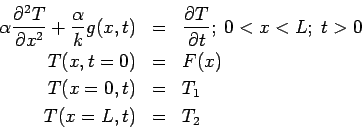
The heat equation descibes transient heat conduction in solids. Consider the following boundary value problem for the temperature in a one-dimensional plate:

$$\begin{eqnarray*} \alpha \frac{\partial ^{2}T}{\partial x^{2}}+\frac{\alpha }{k}... ...\\ T(x,t=0) &=&F(x) \\ T(x=0,t) &=&T_{1} \\ T(x=L,t) &=&T_{2} \end{eqnarray*}$$

Here we seek the temperature $T(x,t)$ (units: Kelvin) in a one-dimensional plate $(0<x<L;\;t>0)$ caused by a specified energy generation function $% g(x,t)$ (units: Watts/m$^{3}$) inside the body. Initially the temperature is a known function $F(x)$. Refer to the figure for the geometry.

Figure: Geometry for transient one-dimensional example.

The thermal properties are conductivity $k$ ($% W/m/K$) and diffusivity $\alpha$ $(m^{2}/\sec )$. Since this is a second order equation two boundary conditions are needed, and in this example at each boundary the temperature is specified (Dirichlet, or type 1, boundary conditions). Other types of boundary conditions are possible.

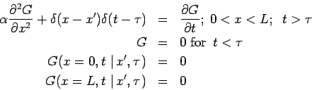
The temperature that satisifies the above equations will be found in two steps. First the GF will be defined, and then the GF will be used to construct the temperature. The Green's function $G\left( x,t\,\left\vert \,x^{\prime },\tau \right. \right)$ associated with the above example obeys the following equations:

$$\begin{eqnarray*} \alpha \frac{\partial ^{2}G}{\partial x^{2}}+\delta (x-x^{\pri... ...) &=&0 \\ G(x=L,t\,\left\vert \,x^{\prime },\tau \right. ) &=&0 \end{eqnarray*}$$

Note that the boundary conditions are of the same type as the temperature problem, but homogeneous, and that the energy generation term has been replaced by a product of two Dirac delta functions $\delta (x-x^{\prime })\delta (t-\tau )$, one for space and one for time. The units of $G$ are determined by the units of the Dirac delta function, and in this 1-D Cartesian case $\left[ G\right] =meters^{-1}$. The Green's function $G\left( x,t\,\left\vert \,x^{\prime },\tau \right. \right)$ represents the temperature response observed at point $x$ and time $t$ caused by an instantaneous concentrated heat source released at point $x^{\prime}$ and time $\tau$. Green's functions are causal since there is no response before the heat source is released: $G=0$ for $t-\tau <0$. Finally, the thermal properties are constant so the differential equation is linear; this is important since the Green's functions may only be found for linear differential equations.

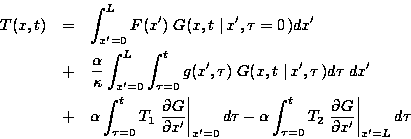
The temperature solution is constructed from a suitable distribution of the GF within the body so as to reproduce the heating conditions. The temperature for this example is given by:

$$\begin{eqnarray*} T(x,t) &=& \int^L_{x^{\prime}=0} F(x^{\prime}) \; G(x,t\,\left... ...tial x^{\prime} } \right\vert _{x^{\prime}=L} d \tau \nonumber \end{eqnarray*}$$

In this temperature expression there is a separate additive term associated with each non-zero heating term: the initial condition; the energy generation; and, one term for each boundary. See ``GF Solution Equation'' for a general discussion of transient temperature described by the GF method.